
官方文件翻譯版(2021/03/31) 原文
未翻譯的部分先把原文搬過來,會慢慢進行更新~
此文章為新手面向的pandas簡短介紹,更詳細的說明可以查看此文件(官方原文)。
詳細說明的文件不可能翻譯的 ><
一般來說起手式為:
In [1]: import numpy as np

In [2]: import pandas as pd
物件的建立
詳細請查看資料結構介紹(官方原文)。
首先讓我們先來產生一個Series,給他一個陣列,他會自行建立對應的數值索引:
In [3]: s = pd.Series([1, 3, 5, np.nan, 6, 8])

In [4]: s
Out[4]:
0    1.0
1    3.0
2    5.0
3    NaN
4    6.0
5    8.0
dtype: float64
再來產生一個DataFrame,給他一個NumPy的陣列:
In [5]: dates = pd.date_range("20130101", periods=6)

In [6]: dates
Out[6]:
DatetimeIndex(['2013-01-01', '2013-01-02', '2013-01-03', '2013-01-04',
 '2013-01-05', '2013-01-06'],
 dtype='datetime64[ns]', freq='D')
再來指定他的索引為日期並且替欄位命名:
In [7]: df = pd.DataFrame(np.random.randn(6, 4), index=dates, columns=list("ABCD"))

In [8]: df
Out[8]:
 A         B         C         D
2013-01-01  0.469112 -0.282863 -1.509059 -1.135632
2013-01-02  1.212112 -0.173215  0.119209 -1.044236
2013-01-03 -0.861849 -2.104569 -0.494929  1.071804
2013-01-04  0.721555 -0.706771 -1.039575  0.271860
2013-01-05 -0.424972  0.567020  0.276232 -1.087401
2013-01-06 -0.673690  0.113648 -1.478427  0.524988
或者可以直接用dict直接建立:
In [9]: df2 = pd.DataFrame(
 ...:    {
 ...:        "A": 1.0,
 ...:        "B": pd.Timestamp("20130102"),
 ...:        "C": pd.Series(1, index=list(range(4)), dtype="float32"),
 ...:        "D": np.array([3] * 4, dtype="int32"),
 ...:        "E": pd.Categorical(["test", "train", "test", "train"]),
 ...:        "F": "foo",
 ...:    }
 ...: )
 ...:

In [10]: df2
Out[10]:
 A          B    C  D      E    F
0  1.0 2013-01-02  1.0  3   test  foo
1  1.0 2013-01-02  1.0  3  train  foo
2  1.0 2013-01-02  1.0  3   test  foo
3  1.0 2013-01-02  1.0  3  train  foo
欄位的型別可以不同:
In [11]: df2.dtypes
Out[11]:
A           float64
B    datetime64[ns]
C           float32
D             int32
E          category
F            object
dtype: object
如果你使用的是IPython,會把欄位自動加入Tab自動完成的屬性中,如下:
In [12]: df2.<TAB>  # noqa: E225, E999
df2.A                  df2.bool
df2.abs                df2.boxplot
df2.add                df2.C
df2.add_prefix         df2.clip
df2.add_suffix         df2.columns
df2.align              df2.copy
df2.all                df2.count
df2.any                df2.combine
df2.append             df2.D
df2.apply              df2.describe
df2.applymap           df2.diff
df2.B                  df2.duplicated
依照上方結果顯示,欄位 A, B, C, D 已被設定到Tab自動完成的屬性中,而 E and F 同樣也是,但為了版面整潔,我們還是省略了吧!
資料呈現
詳細資料請查看基礎介紹。
以下示範如何顯示頭尾資料,
前五列資料:
In [13]: df.head()
Out[13]:
 A         B         C         D
2013-01-01  0.469112 -0.282863 -1.509059 -1.135632
2013-01-02  1.212112 -0.173215  0.119209 -1.044236
2013-01-03 -0.861849 -2.104569 -0.494929  1.071804
2013-01-04  0.721555 -0.706771 -1.039575  0.271860
2013-01-05 -0.424972  0.567020  0.276232 -1.087401
最後五列資料:
In [14]: df.tail(3)
Out[14]:
 A         B         C         D
2013-01-04  0.721555 -0.706771 -1.039575  0.271860
2013-01-05 -0.424972  0.567020  0.276232 -1.087401
2013-01-06 -0.673690  0.113648 -1.478427  0.524988
顯示索引及欄位:
In [15]: df.index
Out[15]:
DatetimeIndex(['2013-01-01', '2013-01-02', '2013-01-03', '2013-01-04',
 '2013-01-05', '2013-01-06'],
 dtype='datetime64[ns]', freq='D')

In [16]: df.columns
Out[16]: Index(['A', 'B', 'C', 'D'], dtype='object')
DataFrame.to_numpy() 可以轉換成NumPy格式的基本資料。
但要注意的是,如果你 DataFrame 的欄位有多種型別,對於效能會有很大的影響,主要是因為NumPy和pandas有根本上的不同 ,而且 NumPy 整個陣列只有一個型別, pandas的DataFrames則是每個欄位可以有一個型別。
所以當你呼叫 DataFrame.to_numpy(),pandas 會找一個可以容下所有DataFrame中欄位型別的 NumPy dtype。
最終可能會導致型別會指向Python物件中的object型別。
當欄位的型別全部為浮點數時,DataFrame.to_numpy() 執行速度會很快而且也不需要透過資料複製產生:
In [17]: df.to_numpy()
Out[17]:
array([[ 0.4691, -0.2829, -1.5091, -1.1356],
 [ 1.2121, -0.1732,  0.1192, -1.0442],
 [-0.8618, -2.1046, -0.4949,  1.0718],
 [ 0.7216, -0.7068, -1.0396,  0.2719],
 [-0.425 ,  0.567 ,  0.2762, -1.0874],
 [-0.6737,  0.1136, -1.4784,  0.525 ]])
而欄位包含多型別時, 相對來說DataFrame.to_numpy() 會較消耗資源:
In [18]: df2.to_numpy()
Out[18]:
array([[1.0, Timestamp('2013-01-02 00:00:00'), 1.0, 3, 'test', 'foo'],
 [1.0, Timestamp('2013-01-02 00:00:00'), 1.0, 3, 'train', 'foo'],
 [1.0, Timestamp('2013-01-02 00:00:00'), 1.0, 3, 'test', 'foo'],
 [1.0, Timestamp('2013-01-02 00:00:00'), 1.0, 3, 'train', 'foo']],
 dtype=object)
DataFrame.to_numpy()輸出中 不包含 索引以及欄位的標籤
describe() 顯示簡單的統計資料:
In [19]: df.describe()
Out[19]:
 A         B         C         D
count  6.000000  6.000000  6.000000  6.000000
mean   0.073711 -0.431125 -0.687758 -0.233103
std    0.843157  0.922818  0.779887  0.973118
min   -0.861849 -2.104569 -1.509059 -1.135632
25%   -0.611510 -0.600794 -1.368714 -1.076610
50%    0.022070 -0.228039 -0.767252 -0.386188
75%    0.658444  0.041933 -0.034326  0.461706
max    1.212112  0.567020  0.276232  1.071804
T 將資料轉置:
In [20]: df.T
Out[20]:
 2013-01-01  2013-01-02  2013-01-03  2013-01-04  2013-01-05  2013-01-06
A    0.469112    1.212112   -0.861849    0.721555   -0.424972   -0.673690
B   -0.282863   -0.173215   -2.104569   -0.706771    0.567020    0.113648
C   -1.509059    0.119209   -0.494929   -1.039575    0.276232   -1.478427
D   -1.135632   -1.044236    1.071804    0.271860   -1.087401    0.524988
sort_index 依照坐標軸進行排序:
In [21]: df.sort_index(axis=1, ascending=False)
Out[21]:
 D         C         B         A
2013-01-01 -1.135632 -1.509059 -0.282863  0.469112
2013-01-02 -1.044236  0.119209 -0.173215  1.212112
2013-01-03  1.071804 -0.494929 -2.104569 -0.861849
2013-01-04  0.271860 -1.039575 -0.706771  0.721555
2013-01-05 -1.087401  0.276232  0.567020 -0.424972
2013-01-06  0.524988 -1.478427  0.113648 -0.673690
sort_values 依照欄位的值進行排序:
In [22]: df.sort_values(by="B")
Out[22]:
 A         B         C         D
2013-01-03 -0.861849 -2.104569 -0.494929  1.071804
2013-01-04  0.721555 -0.706771 -1.039575  0.271860
2013-01-01  0.469112 -0.282863 -1.509059 -1.135632
2013-01-02  1.212112 -0.173215  0.119209 -1.044236
2013-01-06 -0.673690  0.113648 -1.478427  0.524988
2013-01-05 -0.424972  0.567020  0.276232 -1.087401
選取
雖然 Python / Numpy 有方便且容易使用的表達式進行資料選取和設定,但建議還是使用優化過的 pandas 方式, 例如:
.at,.iat,.loc和.iloc。
詳細請查看索引編列的文件Indexing and Selecting Data 和 MultiIndex / Advanced Indexing。
取得
在Series選取單一欄位等同於使用df.A:
In [23]: df["A"]
Out[23]:
2013-01-01    0.469112
2013-01-02    1.212112
2013-01-03   -0.861849
2013-01-04    0.721555
2013-01-05   -0.424972
2013-01-06   -0.673690
Freq: D, Name: A, dtype: float64
透過[]可以將資料以列的方式切割:
In [24]: df[0:3]
Out[24]:
                   A         B         C         D
2013-01-01  0.469112 -0.282863 -1.509059 -1.135632
2013-01-02  1.212112 -0.173215  0.119209 -1.044236
2013-01-03 -0.861849 -2.104569 -0.494929  1.071804

In [25]: df["20130102":"20130104"]
Out[25]:
                   A         B         C         D
2013-01-02  1.212112 -0.173215  0.119209 -1.044236
2013-01-03 -0.861849 -2.104569 -0.494929  1.071804
2013-01-04  0.721555 -0.706771 -1.039575  0.271860
透過標籤進行選取
詳細資料請查看Selection by Label。
透過標籤取得跨欄位資料:
In [26]: df.loc[dates[0]]
Out[26]:
A    0.469112
B   -0.282863
C   -1.509059
D   -1.135632
Name: 2013-01-01 00:00:00, dtype: float64
透過標籤取得多軸資料:
In [27]: df.loc[:, ["A", "B"]]
Out[27]:
                   A         B
2013-01-01  0.469112 -0.282863
2013-01-02  1.212112 -0.173215
2013-01-03 -0.861849 -2.104569
2013-01-04  0.721555 -0.706771
2013-01-05 -0.424972  0.567020
2013-01-06 -0.673690  0.113648
透過標籤取得多軸資料並同時將列切割:
In [28]: df.loc["20130102":"20130104", ["A", "B"]]
Out[28]:
                   A         B
2013-01-02  1.212112 -0.173215
2013-01-03 -0.861849 -2.104569
2013-01-04  0.721555 -0.706771
縮小回傳物件範圍:
In [29]: df.loc["20130102", ["A", "B"]]
Out[29]:
A    1.212112
B   -0.173215
Name: 2013-01-02 00:00:00, dtype: float64
取得單一資料:
In [30]: df.loc[dates[0], "A"]
Out[30]: 0.4691122999071863
快速取得單一資料(結果同上面的方法):
In [31]: df.at[dates[0], "A"]
Out[31]: 0.4691122999071863
透過位置選取
詳細請查看Selection by Position。
透過傳遞數值位置取得資料:
In [32]: df.iloc[3]
Out[32]:
A    0.721555
B   -0.706771
C   -1.039575
D    0.271860
Name: 2013-01-04 00:00:00, dtype: float64
類似於numpy/python的方式,透過數值切割資料:
In [33]: df.iloc[3:5, 0:2]
Out[33]:
                   A         B
2013-01-04  0.721555 -0.706771
2013-01-05 -0.424972  0.567020
類似於numpy/python的方式,透過數值清單指定位置:
In [34]: df.iloc[[1, 2, 4], [0, 2]]
Out[34]:
                   A         C
2013-01-02  1.212112  0.119209
2013-01-03 -0.861849 -0.494929
2013-01-05 -0.424972  0.276232
直接切割列取得資料:
In [35]: df.iloc[1:3, :]
Out[35]:
                   A         B         C         D
2013-01-02  1.212112 -0.173215  0.119209 -1.044236
2013-01-03 -0.861849 -2.104569 -0.494929  1.071804
直接切割欄位取得資料:
In [36]: df.iloc[:, 1:3]
Out[36]:
                   B         C
2013-01-01 -0.282863 -1.509059
2013-01-02 -0.173215  0.119209
2013-01-03 -2.104569 -0.494929
2013-01-04 -0.706771 -1.039575
2013-01-05  0.567020  0.276232
2013-01-06  0.113648 -1.478427
直接取得資料:
In [37]: df.iloc[1, 1]
Out[37]: -0.17321464905330858
快速取得單一值(結果同上面的方法):
In [38]: df.iat[1, 1]
Out[38]: -0.17321464905330858
條件式索引
根據單一欄位的值取得資料:
In [39]: df[df["A"] > 0]
Out[39]:
                   A         B         C         D
2013-01-01  0.469112 -0.282863 -1.509059 -1.135632
2013-01-02  1.212112 -0.173215  0.119209 -1.044236
2013-01-04  0.721555 -0.706771 -1.039575  0.271860
於DataFrame中使用條件選取資料:
In [40]: df[df > 0]
Out[40]:
                   A         B         C         D
2013-01-01  0.469112       NaN       NaN       NaN
2013-01-02  1.212112       NaN  0.119209       NaN
2013-01-03       NaN       NaN       NaN  1.071804
2013-01-04  0.721555       NaN       NaN  0.271860
2013-01-05       NaN  0.567020  0.276232       NaN
2013-01-06       NaN  0.113648       NaN  0.524988
透過 isin() 篩選資料:
In [41]: df2 = df.copy()

In [42]: df2["E"] = ["one", "one", "two", "three", "four", "three"]

In [43]: df2
Out[43]:
                   A         B         C         D      E
2013-01-01  0.469112 -0.282863 -1.509059 -1.135632    one
2013-01-02  1.212112 -0.173215  0.119209 -1.044236    one
2013-01-03 -0.861849 -2.104569 -0.494929  1.071804    two
2013-01-04  0.721555 -0.706771 -1.039575  0.271860  three
2013-01-05 -0.424972  0.567020  0.276232 -1.087401   four
2013-01-06 -0.673690  0.113648 -1.478427  0.524988  three

In [44]: df2[df2["E"].isin(["two", "four"])]
Out[44]:
                   A         B         C         D     E
2013-01-03 -0.861849 -2.104569 -0.494929  1.071804   two
2013-01-05 -0.424972  0.567020  0.276232 -1.087401  four
設定
設定新的欄位時,資料會自動對齊索引:
In [45]: s1 = pd.Series([1, 2, 3, 4, 5, 6], index=pd.date_range("20130102", periods=6))

In [46]: s1
Out[46]:
2013-01-02    1
2013-01-03    2
2013-01-04    3
2013-01-05    4
2013-01-06    5
2013-01-07    6
Freq: D, dtype: int64

In [47]: df["F"] = s1
透過標籤設定資料:
In [48]: df.at[dates[0], "A"] = 0
透過位置設定資料:
In [49]: df.iat[0, 1] = 0
使用NumPy陣列設定資料:
In [50]: df.loc[:, "D"] = np.array([5] * len(df))
上述設定後的結果:
In [51]: df
Out[51]:
                   A         B         C  D    F
2013-01-01  0.000000  0.000000 -1.509059  5  NaN
2013-01-02  1.212112 -0.173215  0.119209  5  1.0
2013-01-03 -0.861849 -2.104569 -0.494929  5  2.0
2013-01-04  0.721555 -0.706771 -1.039575  5  3.0
2013-01-05 -0.424972  0.567020  0.276232  5  4.0
2013-01-06 -0.673690  0.113648 -1.478427  5  5.0
使用 where 方式設定資料:
In [52]: df2 = df.copy()

In [53]: df2[df2 > 0] = -df2

In [54]: df2
Out[54]:
                   A         B         C  D    F
2013-01-01  0.000000  0.000000 -1.509059 -5  NaN
2013-01-02 -1.212112 -0.173215 -0.119209 -5 -1.0
2013-01-03 -0.861849 -2.104569 -0.494929 -5 -2.0
2013-01-04 -0.721555 -0.706771 -1.039575 -5 -3.0
2013-01-05 -0.424972 -0.567020 -0.276232 -5 -4.0
2013-01-06 -0.673690 -0.113648 -1.478427 -5 -5.0
遺失的資料
pandas主要使用 np.nan 來代表遺失的資料,
pandas primarily uses the value np.nan to represent missing data. It is by default not included in computations. See the Missing Data section.
Reindexing allows you to change/add/delete the index on a specified axis. This returns a copy of the data.
In [55]: df1 = df.reindex(index=dates[0:4], columns=list(df.columns) + ["E"])

In [56]: df1.loc[dates[0] : dates[1], "E"] = 1

In [57]: df1
Out[57]:
                   A         B         C  D    F    E
2013-01-01  0.000000  0.000000 -1.509059  5  NaN  1.0
2013-01-02  1.212112 -0.173215  0.119209  5  1.0  1.0
2013-01-03 -0.861849 -2.104569 -0.494929  5  2.0  NaN
2013-01-04  0.721555 -0.706771 -1.039575  5  3.0  NaN
To drop any rows that have missing data.
In [58]: df1.dropna(how="any")
Out[58]:
                   A         B         C  D    F    E
2013-01-02  1.212112 -0.173215  0.119209  5  1.0  1.0
Filling missing data.
In [59]: df1.fillna(value=5)
Out[59]:
                   A         B         C  D    F    E
2013-01-01  0.000000  0.000000 -1.509059  5  5.0  1.0
2013-01-02  1.212112 -0.173215  0.119209  5  1.0  1.0
2013-01-03 -0.861849 -2.104569 -0.494929  5  2.0  5.0
2013-01-04  0.721555 -0.706771 -1.039575  5  3.0  5.0
To get the boolean mask where values are nan.
In [60]: pd.isna(df1)
Out[60]:
                A      B      C      D      F      E
2013-01-01  False  False  False  False   True  False
2013-01-02  False  False  False  False  False  False
2013-01-03  False  False  False  False  False   True
2013-01-04  False  False  False  False  False   True
Operations
See the Basic section on Binary Ops.
Stats
Operations in general exclude missing data.
Performing a descriptive statistic:
In [61]: df.mean()
Out[61]:
A   -0.004474
B   -0.383981
C   -0.687758
D    5.000000
F    3.000000
dtype: float64
Same operation on the other axis:
In [62]: df.mean(1)
Out[62]:
2013-01-01    0.872735
2013-01-02    1.431621
2013-01-03    0.707731
2013-01-04    1.395042
2013-01-05    1.883656
2013-01-06    1.592306
Freq: D, dtype: float64
Operating with objects that have different dimensionality and need alignment. In addition, pandas automatically broadcasts along the specified dimension.
In [63]: s = pd.Series([1, 3, 5, np.nan, 6, 8], index=dates).shift(2)

In [64]: s
Out[64]:
2013-01-01    NaN
2013-01-02    NaN
2013-01-03    1.0
2013-01-04    3.0
2013-01-05    5.0
2013-01-06    NaN
Freq: D, dtype: float64

In [65]: df.sub(s, axis="index")
Out[65]:
                   A         B         C    D    F
2013-01-01       NaN       NaN       NaN  NaN  NaN
2013-01-02       NaN       NaN       NaN  NaN  NaN
2013-01-03 -1.861849 -3.104569 -1.494929  4.0  1.0
2013-01-04 -2.278445 -3.706771 -4.039575  2.0  0.0
2013-01-05 -5.424972 -4.432980 -4.723768  0.0 -1.0
2013-01-06       NaN       NaN       NaN  NaN  NaN
Apply
Applying functions to the data:
In [66]: df.apply(np.cumsum)
Out[66]:
                   A         B         C   D     F
2013-01-01  0.000000  0.000000 -1.509059   5   NaN
2013-01-02  1.212112 -0.173215 -1.389850  10   1.0
2013-01-03  0.350263 -2.277784 -1.884779  15   3.0
2013-01-04  1.071818 -2.984555 -2.924354  20   6.0
2013-01-05  0.646846 -2.417535 -2.648122  25  10.0
2013-01-06 -0.026844 -2.303886 -4.126549  30  15.0

In [67]: df.apply(lambda x: x.max() - x.min())
Out[67]:
A    2.073961
B    2.671590
C    1.785291
D    0.000000
F    4.000000
dtype: float64
Histogramming
See more at Histogramming and Discretization.
In [68]: s = pd.Series(np.random.randint(0, 7, size=10))

In [69]: s
Out[69]:
0    4
1    2
2    1
3    2
4    6
5    4
6    4
7    6
8    4
9    4
dtype: int64

In [70]: s.value_counts()
Out[70]:
4    5
2    2
6    2
1    1
dtype: int64
String Methods
Series is equipped with a set of string processing methods in the str attribute that make it easy to operate on each element of the array, as in the code snippet below. Note that pattern-matching in str generally uses regular expressions by default (and in some cases always uses them). See more at Vectorized String Methods.
In [71]: s = pd.Series(["A", "B", "C", "Aaba", "Baca", np.nan, "CABA", "dog", "cat"])

In [72]: s.str.lower()
Out[72]:
0       a
1       b
2       c
3    aaba
4    baca
5     NaN
6    caba
7     dog
8     cat
dtype: object
Merge
Concat
pandas provides various facilities for easily combining together Series and DataFrame objects with various kinds of set logic for the indexes and relational algebra functionality in the case of join / merge-type operations.
See the Merging section.
Concatenating pandas objects together with concat():
In [73]: df = pd.DataFrame(np.random.randn(10, 4))

In [74]: df
Out[74]:
          0         1         2         3
0 -0.548702  1.467327 -1.015962 -0.483075
1  1.637550 -1.217659 -0.291519 -1.745505
2 -0.263952  0.991460 -0.919069  0.266046
3 -0.709661  1.669052  1.037882 -1.705775
4 -0.919854 -0.042379  1.247642 -0.009920
5  0.290213  0.495767  0.362949  1.548106
6 -1.131345 -0.089329  0.337863 -0.945867
7 -0.932132  1.956030  0.017587 -0.016692
8 -0.575247  0.254161 -1.143704  0.215897
9  1.193555 -0.077118 -0.408530 -0.862495

# break it into pieces
In [75]: pieces = [df[:3], df[3:7], df[7:]]

In [76]: pd.concat(pieces)
Out[76]:
          0         1         2         3
0 -0.548702  1.467327 -1.015962 -0.483075
1  1.637550 -1.217659 -0.291519 -1.745505
2 -0.263952  0.991460 -0.919069  0.266046
3 -0.709661  1.669052  1.037882 -1.705775
4 -0.919854 -0.042379  1.247642 -0.009920
5  0.290213  0.495767  0.362949  1.548106
6 -1.131345 -0.089329  0.337863 -0.945867
7 -0.932132  1.956030  0.017587 -0.016692
8 -0.575247  0.254161 -1.143704  0.215897
9  1.193555 -0.077118 -0.408530 -0.862495
Adding a column to a DataFrame is relatively fast. However, adding a row requires a copy, and may be expensive. We recommend passing a pre-built list of records to the DataFrame constructor instead of building a DataFrame by iteratively appending records to it. See Appending to dataframe for more.
Join
SQL style merges. See the Database style joining section.
In [77]: left = pd.DataFrame({"key": ["foo", "foo"], "lval": [1, 2]})

In [78]: right = pd.DataFrame({"key": ["foo", "foo"], "rval": [4, 5]})

In [79]: left
Out[79]:
   key  lval
0  foo     1
1  foo     2

In [80]: right
Out[80]:
   key  rval
0  foo     4
1  foo     5

In [81]: pd.merge(left, right, on="key")
Out[81]:
   key  lval  rval
0  foo     1     4
1  foo     1     5
2  foo     2     4
3  foo     2     5
Another example that can be given is:
In [82]: left = pd.DataFrame({"key": ["foo", "bar"], "lval": [1, 2]})

In [83]: right = pd.DataFrame({"key": ["foo", "bar"], "rval": [4, 5]})

In [84]: left
Out[84]:
   key  lval
0  foo     1
1  bar     2

In [85]: right
Out[85]:
   key  rval
0  foo     4
1  bar     5

In [86]: pd.merge(left, right, on="key")
Out[86]:
   key  lval  rval
0  foo     1     4
1  bar     2     5
Grouping
By “group by” we are referring to a process involving one or more of the following steps:
- Splitting the data into groups based on some criteria
- Applying a function to each group independently
- Combining the results into a data structure
See the Grouping section.
In [87]: df = pd.DataFrame(
   ....:     {
   ....:         "A": ["foo", "bar", "foo", "bar", "foo", "bar", "foo", "foo"],
   ....:         "B": ["one", "one", "two", "three", "two", "two", "one", "three"],
   ....:         "C": np.random.randn(8),
   ....:         "D": np.random.randn(8),
   ....:     }
   ....: )
   ....:

In [88]: df
Out[88]:
     A      B         C         D
0  foo    one  1.346061 -1.577585
1  bar    one  1.511763  0.396823
2  foo    two  1.627081 -0.105381
3  bar  three -0.990582 -0.532532
4  foo    two -0.441652  1.453749
5  bar    two  1.211526  1.208843
6  foo    one  0.268520 -0.080952
7  foo  three  0.024580 -0.264610
Grouping and then applying the sum() function to the resulting groups.
In [89]: df.groupby("A").sum()
Out[89]:
            C         D
A
bar  1.732707  1.073134
foo  2.824590 -0.574779
Grouping by multiple columns forms a hierarchical index, and again we can apply the sum() function.
In [90]: df.groupby(["A", "B"]).sum()
Out[90]:
                  C         D
A   B
bar one    1.511763  0.396823
    three -0.990582 -0.532532
    two    1.211526  1.208843
foo one    1.614581 -1.658537
    three  0.024580 -0.264610
    two    1.185429  1.348368
Reshaping
See the sections on Hierarchical Indexing and Reshaping.
Stack
In [91]: tuples = list(
   ....:     zip(
   ....:         *[
   ....:             ["bar", "bar", "baz", "baz", "foo", "foo", "qux", "qux"],
   ....:             ["one", "two", "one", "two", "one", "two", "one", "two"],
   ....:         ]
   ....:     )
   ....: )
   ....:

In [92]: index = pd.MultiIndex.from_tuples(tuples, names=["first", "second"])

In [93]: df = pd.DataFrame(np.random.randn(8, 2), index=index, columns=["A", "B"])

In [94]: df2 = df[:4]

In [95]: df2
Out[95]:
                     A         B
first second
bar   one    -0.727965 -0.589346
      two     0.339969 -0.693205
baz   one    -0.339355  0.593616
      two     0.884345  1.591431
The stack() method “compresses” a level in the DataFrame’s columns.
In [96]: stacked = df2.stack()

In [97]: stacked
Out[97]:
first  second
bar    one     A   -0.727965
               B   -0.589346
       two     A    0.339969
               B   -0.693205
baz    one     A   -0.339355
               B    0.593616
       two     A    0.884345
               B    1.591431
dtype: float64
With a “stacked” DataFrame or Series (having a MultiIndex as the index), the inverse operation of stack() is unstack(), which by default unstacks the last level:
In [98]: stacked.unstack()
Out[98]:
                     A         B
first second
bar   one    -0.727965 -0.589346
      two     0.339969 -0.693205
baz   one    -0.339355  0.593616
      two     0.884345  1.591431

In [99]: stacked.unstack(1)
Out[99]:
second        one       two
first
bar   A -0.727965  0.339969
      B -0.589346 -0.693205
baz   A -0.339355  0.884345
      B  0.593616  1.591431

In [100]: stacked.unstack(0)
Out[100]:
first          bar       baz
second
one    A -0.727965 -0.339355
       B -0.589346  0.593616
two    A  0.339969  0.884345
       B -0.693205  1.
Pivot tables
See the section on Pivot Tables.
In [101]: df = pd.DataFrame(
   .....:     {
   .....:         "A": ["one", "one", "two", "three"] * 3,
   .....:         "B": ["A", "B", "C"] * 4,
   .....:         "C": ["foo", "foo", "foo", "bar", "bar", "bar"] * 2,
   .....:         "D": np.random.randn(12),
   .....:         "E": np.random.randn(12),
   .....:     }
   .....: )
   .....:

In [102]: df
Out[102]:
        A  B    C         D         E
0     one  A  foo -1.202872  0.047609
1     one  B  foo -1.814470 -0.136473
2     two  C  foo  1.018601 -0.561757
3   three  A  bar -0.595447 -1.623033
4     one  B  bar  1.395433  0.029399
5     one  C  bar -0.392670 -0.542108
6     two  A  foo  0.007207  0.282696
7   three  B  foo  1.928123 -0.087302
8     one  C  foo -0.055224 -1.575170
9     one  A  bar  2.395985  1.771208
10    two  B  bar  1.552825  0.816482
11  three  C  bar  0.166599  1.100230
We can produce pivot tables from this data very easily:
In [103]: pd.pivot_table(df, values="D", index=["A", "B"], columns=["C"])
Out[103]:
C             bar       foo
A     B
one   A  2.395985 -1.202872
      B  1.395433 -1.814470
      C -0.392670 -0.055224
three A -0.595447       NaN
      B       NaN  1.928123
      C  0.166599       NaN
two   A       NaN  0.007207
      B  1.552825       NaN
      C       NaN  1.018601
Time series
pandas has simple, powerful, and efficient functionality for performing resampling operations during frequency conversion (e.g., converting secondly data into 5-minutely data). This is extremely common in, but not limited to, financial applications. See the Time Series section.
In [105]: ts = pd.Series(np.random.randint(0, 500, len(rng)), index=rng)

In [106]: ts.resample("5Min").sum()
Out[106]:
2012-01-01    24182
Freq: 5T, dtype: int64
Time zone representation:
In [107]: rng = pd.date_range("3/6/2012 00:00", periods=5, freq="D")

In [108]: ts = pd.Series(np.random.randn(len(rng)), rng)

In [109]: ts
Out[109]:
2012-03-06    1.857704
2012-03-07   -1.193545
2012-03-08    0.677510
2012-03-09   -0.153931
2012-03-10    0.520091
Freq: D, dtype: float64

In [110]: ts_utc = ts.tz_localize("UTC")

In [111]: ts_utc
Out[111]:
2012-03-06 00:00:00+00:00    1.857704
2012-03-07 00:00:00+00:00   -1.193545
2012-03-08 00:00:00+00:00    0.677510
2012-03-09 00:00:00+00:00   -0.153931
2012-03-10 00:00:00+00:00    0.520091
Freq: D, dtype: float64
Converting to another time zone:

In [112]: ts_utc.tz_convert("US/Eastern")
Out[112]:
2012-03-05 19:00:00-05:00    1.857704
2012-03-06 19:00:00-05:00   -1.193545
2012-03-07 19:00:00-05:00    0.677510
2012-03-08 19:00:00-05:00   -0.153931
2012-03-09 19:00:00-05:00    0.520091
Freq: D, dtype: float64
Converting between time span representations:
In [113]: rng = pd.date_range("1/1/2012", periods=5, freq="M")

In [114]: ts = pd.Series(np.random.randn(len(rng)), index=rng)

In [115]: ts
Out[115]:
2012-01-31   -1.475051
2012-02-29    0.722570
2012-03-31   -0.322646
2012-04-30   -1.601631
2012-05-31    0.778033
Freq: M, dtype: float64

In [116]: ps = ts.to_period()

In [117]: ps
Out[117]:
2012-01   -1.475051
2012-02    0.722570
2012-03   -0.322646
2012-04   -1.601631
2012-05    0.778033
Freq: M, dtype: float64

In [118]: ps.to_timestamp()
Out[118]:
2012-01-01   -1.475051
2012-02-01    0.722570
2012-03-01   -0.322646
2012-04-01   -1.601631
2012-05-01    0.778033
Freq: MS, dtype: float64
Converting between period and timestamp enables some convenient arithmetic functions to be used. In the following example, we convert a quarterly frequency with year ending in November to 9am of the end of the month following the quarter end:
In [119]: prng = pd.period_range("1990Q1", "2000Q4", freq="Q-NOV")

In [120]: ts = pd.Series(np.random.randn(len(prng)), prng)

In [121]: ts.index = (prng.asfreq("M", "e") + 1).asfreq("H", "s") + 9

In [122]: ts.head()
Out[122]:
1990-03-01 09:00   -0.289342
1990-06-01 09:00    0.233141
1990-09-01 09:00   -0.223540
1990-12-01 09:00    0.542054
1991-03-01 09:00   -0.688585
Freq: H, dtype: float64
Categoricals
pandas can include categorical data in a DataFrame. For full docs, see the categorical introduction and the API documentation.
In [123]: df = pd.DataFrame(
   .....:     {"id": [1, 2, 3, 4, 5, 6], "raw_grade": ["a", "b", "b", "a", "a", "e"]}
   .....: )
   .....:
Convert the raw grades to a categorical data type.
In [124]: df["grade"] = df["raw_grade"].astype("category")

In [125]: df["grade"]
Out[125]:
0    a
1    b
2    b
3    a
4    a
5    e
Name: grade, dtype: category
Categories (3, object): ['a', 'b', 'e']
Rename the categories to more meaningful names (assigning to Series.cat.categories() is in place!).
In [126]: df["grade"].cat.categories = ["very good", "good", "very bad"]
Reorder the categories and simultaneously add the missing categories (methods under Series.cat() return a new Series by default).
In [127]: df["grade"] = df["grade"].cat.set_categories(
   .....:     ["very bad", "bad", "medium", "good", "very good"]
   .....: )
   .....:

In [128]: df["grade"]
Out[128]:
0    very good
1         good
2         good
3    very good
4    very good
5     very bad
Name: grade, dtype: category
Categories (5, object): ['very bad', 'bad', 'medium', 'good', 'very good']
Sorting is per order in the categories, not lexical order.
In [129]: df.sort_values(by="grade")
Out[129]:
   id raw_grade      grade
5   6         e   very bad
1   2         b       good
2   3         b       good
0   1         a  very good
3   4         a  very good
4   5         a  very good
Grouping by a categorical column also shows empty categories.
In [130]: df.groupby("grade").size()
Out[130]:
grade
very bad     1
bad          0
medium       0
good         2
very good    3
dtype: int64
Plotting
See the Plotting docs.
We use the standard convention for referencing the matplotlib API:
In [131]: import matplotlib.pyplot as plt

In [132]: plt.close("all")
In [133]: ts = pd.Series(np.random.randn(1000), index=pd.date_range("1/1/2000", periods=1000))

In [134]: ts = ts.cumsum()

In [135]: ts.plot()
Out[135]: <AxesSubplot:>
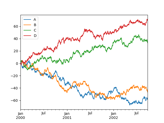
On a DataFrame, the plot() method is a convenience to plot all of the columns with labels:
In [136]: df = pd.DataFrame(
   .....:     np.random.randn(1000, 4), index=ts.index, columns=["A", "B", "C", "D"]
   .....: )
   .....:

In [137]: df = df.cumsum()

In [138]: plt.figure()
Out[138]: <Figure size 640x480 with 0 Axes>

In [139]: df.plot()
Out[139]: <AxesSubplot:>

In [140]: plt.legend(loc='best')
Out[140]: <matplotlib.legend.Legend at 0x7fd2f7ba9580>
Getting data in/out
CSV
In [141]: df.to_csv("foo.csv")
In [142]: pd.read_csv("foo.csv")
Out[142]:
     Unnamed: 0          A          B          C          D
0    2000-01-01   0.350262   0.843315   1.798556   0.782234
1    2000-01-02  -0.586873   0.034907   1.923792  -0.562651
2    2000-01-03  -1.245477  -0.963406   2.269575  -1.612566
3    2000-01-04  -0.252830  -0.498066   3.176886  -1.275581
4    2000-01-05  -1.044057   0.118042   2.768571   0.386039
..          ...        ...        ...        ...        ...
995  2002-09-22 -48.017654  31.474551  69.146374 -47.541670
996  2002-09-23 -47.207912  32.627390  68.505254 -48.828331
997  2002-09-24 -48.907133  31.990402  67.310924 -49.391051
998  2002-09-25 -50.146062  33.716770  67.717434 -49.037577
999  2002-09-26 -49.724318  33.479952  68.108014 -48.822030

[1000 rows x 5 columns
HDF5
Reading and writing to HDFStores.
Writing to a HDF5 Store.
In [143]: df.to_hdf("foo.h5", "df")
Reading from a HDF5 Store.
In [144]: pd.read_hdf("foo.h5", "df")
Out[144]:
                    A          B          C          D
2000-01-01   0.350262   0.843315   1.798556   0.782234
2000-01-02  -0.586873   0.034907   1.923792  -0.562651
2000-01-03  -1.245477  -0.963406   2.269575  -1.612566
2000-01-04  -0.252830  -0.498066   3.176886  -1.275581
2000-01-05  -1.044057   0.118042   2.768571   0.386039
...               ...        ...        ...        ...
2002-09-22 -48.017654  31.474551  69.146374 -47.541670
2002-09-23 -47.207912  32.627390  68.505254 -48.828331
2002-09-24 -48.907133  31.990402  67.310924 -49.391051
2002-09-25 -50.146062  33.716770  67.717434 -49.037577
2002-09-26 -49.724318  33.479952  68.108014 -48.822030

[1000 rows x 4 columns]
Excel
Reading and writing to MS Excel.
Writing to an excel file.
In [145]: df.to_excel("foo.xlsx", sheet_name="Sheet1")
Reading from an excel file.
In [146]: pd.read_excel("foo.xlsx", "Sheet1", index_col=None, na_values=["NA"])
Out[146]:
    Unnamed: 0          A          B          C          D
0   2000-01-01   0.350262   0.843315   1.798556   0.782234
1   2000-01-02  -0.586873   0.034907   1.923792  -0.562651
2   2000-01-03  -1.245477  -0.963406   2.269575  -1.612566
3   2000-01-04  -0.252830  -0.498066   3.176886  -1.275581
4   2000-01-05  -1.044057   0.118042   2.768571   0.386039
..         ...        ...        ...        ...        ...
995 2002-09-22 -48.017654  31.474551  69.146374 -47.541670
996 2002-09-23 -47.207912  32.627390  68.505254 -48.828331
997 2002-09-24 -48.907133  31.990402  67.310924 -49.391051
998 2002-09-25 -50.146062  33.716770  67.717434 -49.037577
999 2002-09-26 -49.724318  33.479952  68.108014 -48.822030

[1000 rows x 5 columns]
Gotchas
If you are attempting to perform an operation you might see an exception like:
>>> if pd.Series([False, True, False]):
...     print("I was true")
Traceback
    ...
ValueError: The truth value of an array is ambiguous. Use a.empty, a.any() or a.all().
See Comparisons for an explanation and what to do.
See Gotchas as well.
